
an in-depth analysis of the architecture and inverse kinematics
Note: The downloadable PDF includes references not available in the web version.
Introduction
The goal of this paper is to lay-out our methodology to create our physical robotic arm, simulated robotic arm and programming environment, made as an end project for “The Lab”, a course in our study of Applied Computer Science. The intention behind this project was to end up with a palpable result that encompasses all layers of a system from hardware to software after applying all the knowledge that we have gathered over the years at KdG University of Applied Sciences and Arts. To not go out of scope or present irrelevant information, this study will only cover an in-depth analysis of the complete architecture and the specific kinematics used for our robotic arm. Lastly, to get the most out of this study, it is recommended to be familiar with concepts like basic robotics, 3D space, kinematics and matrices.
Architecture
In the introduction to this paper, we have mentioned that our project encompasses all system layers. In this section, we will work from the bottom up and give a thorough explanation of the functionality utilised on each one.
Hardware
The actual creation of the physical arm was done outside of project hours and thus, is not officially part of the project. However, it is essential to have a general idea of the machine and its components to have sufficient context to understand the rest of this paper. Therefore, we will give a brief overview of the physical arm.
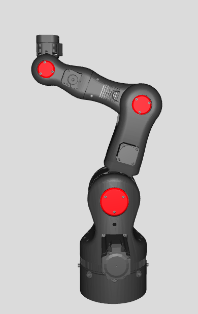
The first step in the creation of the arm was designing it. Our robotic arm is based on the open-source 3D printed robotic arm, the BCN3D Moveo, created by BCN3D Technologies. After tweaking the design a bit further in a computer-aided design (CAD) program, we had our robotic arm ready for production. The result can be seen in the following figure.
One of our objectives was to make the arm move along the x, y and z-axis and to make it rotate in three dimensions: yaw, pitch and roll. For each of these movements, a separate joint is needed, resulting in our robotic arm consisting of six joints in total. Looking at the figure, the rotating disk at the base of the arm is the joint that allows movement along the y-axis. The two joints above the disk work conjointly, mainly for movement along the x and z-axis. Perhaps unexpectedly, the next joint is not the following similar-looking part, but a less visible joint in between these. This joint decides the roll, while the following joint decides the pitch. The last joint, which controls the yaw, is integrated into the end effector.
Moreover, we also created three physical buttons with each their own functionality. One to start the currently active routine, one to swap the current routine with a new one, and an emergency stop button.
Firmware
Most firmware runs on a Raspberry Pi 5. All functionality running on this component is written in Python. The Raspberry Pi is responsible for calculating the necessary angles for the different joints of the arm through inverse kinematics, as well as the velocity at which the joints should move. We need a separate component for this because the microcontroller alone is not performant enough to do all these calculations accurately and quickly enough. To obtain the necessary data for the kinematics, the Raspberry Pi parses YAML configuration files using Pydantic. Pydantic is the most widely used data validation library for Python (Welcome To Pydantic – Pydantic, z.d.). Afterwards, it passes these angles and the velocity to the microcontroller.
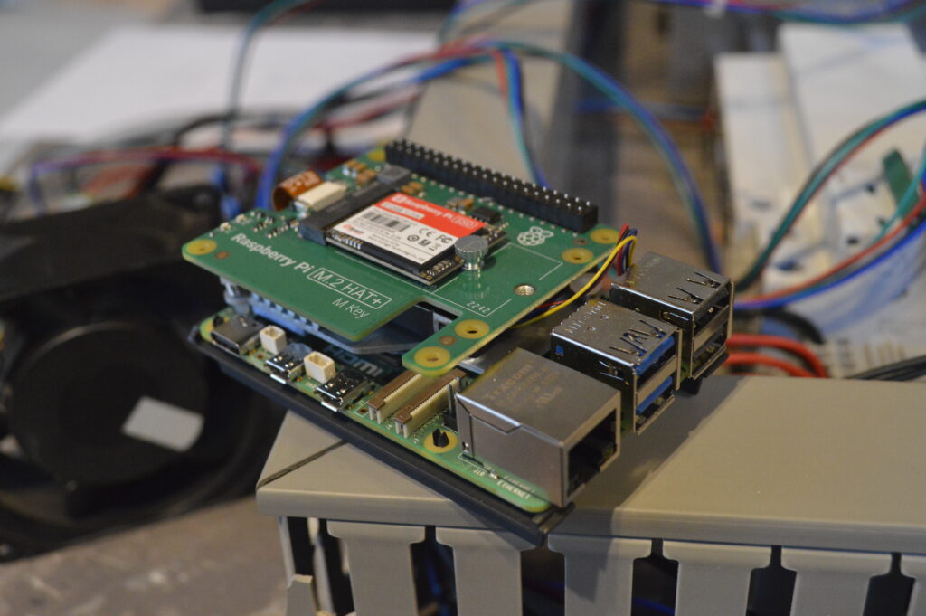
Additionally, this unit runs a web server with FastApi to manage the connection between the physical arm and the application on the PC. FastAPI is a modern, fast (high-performance), web framework for building APIs with Python based on standard Python type hints (FastAPI, z.d.). The software from the PC can send instructions over to this web server, where they get stored in a buffer. When pressing the swap button, the program will swap the currently active routine with the routine stored in the buffer. Pressing the start button afterwards will start the new routine.
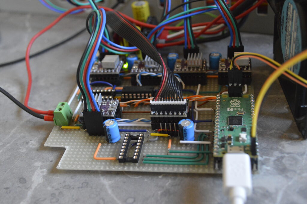
The microcontroller, a Raspberry Pi Pico, receives the angles for the different joints calculated by the Raspberry Pi 5 plus the velocity at which the motors should move. It will pass on these instructions to each motor. All of this is written in C as this is a common choice for low-level programming, and we already had experience with the language.
Software
The software can be divided into two parts. First is the programming environment, where users can create routines to be executed by either the simulated robotic arm or the physical one and second is the simulation, which consists of the actual rendering of the 3D model and its animations and the inverse kinematics needed for this. This allows users to utilise our application even without access to a physical arm or just to test created routines before truly sending it to the physical unit. Due to computer graphics’ reputation for heavily leveraging memory management, our programming of choice is C++, an efficient language that allows for detailed memory management. Moreover, the majority of graphics libraries work with C++.
Simulation
To render the environment and 3D model, we used OpenGL. OpenGL is the name for the specification that describes the behaviour of a rasterization-based rendering system. It defines the API through which a client application can control this system. Our simulation specifically used an OpenGL library called GLFW 3.4. GLFW is an Open Source, multi-platform library for OpenGL, OpenGL ES and Vulkan development on the desktop. It provides a simple API for creating windows, contexts and surfaces, receiving input and events. Furthermore, to load needed OpenGL extensions, we used GLEW 1.13. The OpenGL Extension Wrangler Library is a cross-platform open-source C/C++ extension loading library. GLEW provides efficient run-time mechanisms for determining which OpenGL extensions are supported on the target platform. Finally, as computer graphics regularly utilise matrices for tasks like rendering and perform different calculations with these, we used OpenGL Mathematics. OpenGL Mathematics is a header only C++ mathematics library for graphics software based on the OpenGL Shading Language specifications. This combination of libraries made for a cross-platform OpenGL application with the necessary functionality to create our desired simulated environment.
The figure displays the 3D model that we used in our project, a one-on-one replica of our physical unit. Importing the model into our simulation was not difficult, since we based our arm on the existing BCN3D Moveo. This open-source project already contained files for 3D rendering, so we only had to update them with the changes we made in our physical model. The aforementioned graphics libraries finally imported these files and made the model ready for use.
Programming environment
The goal of the programming environment is to provide an intuitive interface for creating routines for the robotic arm. Furthermore, we wanted to make it useable regardless of programming knowledge. That is why we opted for a block-based approach. This way, instructions made by the user would be independent of the backend implementation. The user only has to choose from a variety of instruction nodes and input the required parameters for it to work.

As you can see, there is a window listing all the possible types of nodes. Most of these have parameters that the user needs to fill in. To create an actual routine with multiple nodes, the user will need to select and place these nodes, fill in the required parameters and link them in the order of execution. Once the user has done this and wants to execute the routine, they can either choose to send it to the simulation or the physical unit by clicking the corresponding button. Otherwise, the user can choose to save this configuration or to load another one. Furthermore, there is an information window that gives the user additional information, e.g. error messages.
To create this user interface, we used Dear ImGui, a self-contained, renderer-agnostic graphics library for C++. The initial reason why we even looked at this library was because we had already heard of it before, but never used it. We eventually decided on ImGui for several reasons. Firstly, ImGui is compatible with OpenGL, which is essential for it to be properly integrated into our project. Secondly, it is self-contained, meaning that it has no external dependencies. Therefore, we already avoided issues with incompatible versions of libraries or libraries that are not available on all operating systems. Finally, Dear ImGui provides a clean, simplistic interface, which we found fitting for the overall aesthetics of our application.
To assist us in creating our programming environment within the timeframe of this course, we used a premade node editor for the Dear ImGui library. This editor took care of many interactions in the environment for us. What we did was interpret the inputs that the node editor received and connect this component to the rest of our application.
One important further feature we implemented to significantly improve the quality of life is the ability to save and load a routine created in the editor. This saves a substantial amount of time by not having to recreate a whole routine every time you use the application and allows you to easily switch between multiple routines.
Miscellaneous
Additionally, the project contains a YAML parser. Originally, this parser was used to handle configuration files that held all sorts of data about the robotic arm. Later, most of this functionality was moved to ini files with its own parser, because this format was more fitting to structure the data needed to render the arm. However, it is still used in certain places within our software.
For the software to be able to connect to the physical arm, we send POST requests to the web server running on the Raspberry Pi containing the necessary G-code, a popular 3D printing programming language. Sending these requests is done with the help of the curlpp wrapper of the libcurl library, a popular URL transfer library in C++. The complete process goes as follows, we first translate all the instructions assigned to the arm to the corresponding G-code and then send it over to the physical unit, where the G-code gets parsed into instructions that can be sent to the microcontroller. Although not actively used in the final version of our project, functionality to save the arm’s current routine to G-code in a file or load G-code from a file into the application has been implemented as well.
Kinematics
One of the core aspects of this project was the kinematics. This paper has mentioned them several times already, thus you will likely have a general idea of what these are, but we wanted to give a more thorough explanation about this subfield of physics and mathematics that played a key role both in the physical side and the simulated one. The focus of this chapter will be on how we applied kinematics to our project, and not on the actual calculations.
Firstly, we need to differentiate between the two types of kinematics. Using the angles of the joints to calculate the coordinates of the arm’s current position is called forward kinematics. Starting from the coordinates of the current position and calculating the angle of each joint needed to achieve this position is called inverse kinematics. Both cases require you to go through a complex mathematical process that is prone to error.
Forward kinematics
Due to only knowing the angles of the joints at startup, we use forward kinematics to find the initial position of the arm. The actual calculations are simpler than those of the inverse kinematics because it is mostly just multiplying the transformation matrices of the joints. We initially used the numpy package to do these calculations in Python, but we had a loss of accuracy that exceeded the acceptable threshold. For that reason, we switched to the sympy package. Sympy is a lot slower but makes up for it with a significant increase in accuracy and as we only use it once at startup, this amount of latency is acceptable.
Inverse kinematics
Inverse kinematics are used repeatedly in both the firmware for the physical arm and the simulation. It’s the key factor for every movement the arm performs. With such a complex system as a robotic arm, that can move along multiple axes and perform different rotations as well, even a simple movement requires a substantial amount of synergy between all parts. Every component needs to execute its instruction with enough accuracy and the correct timing.
The first step is to find the spherical wrist of the arm, which is located in the fifth joint. Using matrix multiplications, we can work our way back from the position we started with to the position of the spherical wrist. The next step is to use trigonometric formulas to calculate the angles of the first, second and third joints. After doing that, we use these angles to discover the position of the third joint in space, similar to the forward kinematics.
While the first, second and third joints dictate the translation, the fourth, fifth and sixth joints dictate the rotation of the wrist. Thus, after obtaining the transformation matrix for the position of the third joint, we only need the part that defines its rotation. Afterwards, we need to “subtract” the rotation of the third joint from the overall rotation of the arm to find the matrix defining the yaw, pitch and roll of the wrist. Using trigonometry once again, we can then find the angles for the last three joints.
The inverse kinematics for the physical arm were done on the Raspberry Pi 5, after receiving the instructions on the webserver. The calculations were made in Python with the use of the numpy package. Contrary to the situation with the forward kinematics, this time the accuracy was acceptable and because the inverse kinematics were used frequently, speed was of the essence. The inverse kinematics for the simulation were done in C++ with the use of the GLM library, which specialises in matrix computations.
Challenges
Solving such a complex problem can be quite challenging. Firstly, understanding the theory behind it already requires a certain level of mathematical insight. Secondly, as you might have noticed from the explanation already, the equations are highly dependent on the type of robotic arm you use.
For example, if your arm has another amount of joints, the equations will be completely different. It is not possible to use the same calculations of a unit with six joints for a unit with three joints. Moreover, you need precise measurements for your robotic arm as well. Fortunately, we used calculations that utilise Denavit–Hartenberg parameters. These parameters allow you to pass on your measurements as variables in the different equations, meaning that if you wanted to use a different arm (with the constraint of having the same amount of joints) you only have to pass the measurements as Denavit-Hartenberg parameters to the equations for it to work.
Another problem that we ran into is that the equations work with the centre of a joint. In reality, the joint is an object with a certain volume with the consequence that even if the kinematics decide that a certain position is theoretically reachable, the volumes of the different components might conflict, e.g. in the simulation, it would cause the model to clip through itself. For that reason, it was important to add extra methods that consider this and place the necessary limits on the joints.
Lastly, a challenge we encountered was that the arm obviously cannot teleport, but has to travel a route to get to their destination. Just calculating the angles for the joints for the destination is not enough. We had to interpolate between the starting position and the end position and apply the inverse kinematics to every interpolated point. Of course, this therefore meant that we had to handle cases where one or more interpolated points may not have been reachable, but the end position was, or the other way around.
Conclusion
This study has provided a comprehensive overview of the development process for this project, detailing the methodologies and tools employed to achieve our objectives. The discussion was structured in two key parts: first, an in-depth analysis of each system layer, outlining our goal for each part, the selected technologies, and the reasons behind our decisions; and second, an exploration of kinematics, a fundamental concept in robotics. Beyond the technical insights gained, this project also offered valuable experience in team collaboration and large-scale project management.